Effect Inputs
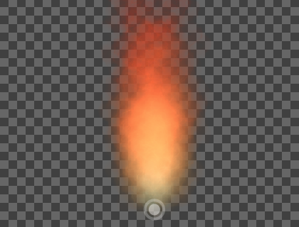
When creating any type of visual effect in games, you are going to encounter the need to dynamically change the effect depending on the current game state. For example, you may want to increase or decrease the scale and intensity of a flame effect based on the situation in the game. This could be done by individually changing all necessary particle properties such as particle count, particle velocity and color. However, this is a task that should be ideally be done during the design phase of the effect. Effect inputs offer exactly this capability. You can define high-level effect attributes or inputs like Intensity and connect them to effect properties via compute graphs, a visual scripting language. The following pictures show how a flame effect could look like with different values for the Intensity input.

Managing effect inputs
Effect inputs are high-level attributes to allow effects to react dynamically to changing situations. They can be booleans, integers, numbers and vectors. You can manage these inputs in the Inputs window.
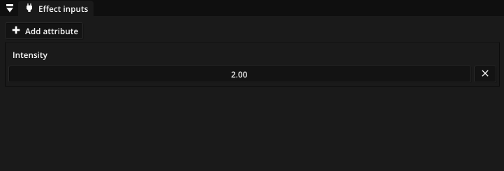
Add a new effect input by clicking the Add attribute. You can choose from different data types.
Data type |
Description |
|---|---|
Boolean |
The input can be true or false, which is useful for toggling things on and off. |
Integer |
The input is a positive or negative number without fractions. |
Number |
The input is a positive or negative number with fractions. |
Vector 2 |
The input is a two-dimensional vector of positive or negative numbers with fractions. Useful for representing 2D positions and directions. |
Vector 3 |
The input is a three-dimensional vector of positive or negative numbers with fractions. Useful for representing 3D positions, directions and colors. |
Vector 4 |
The input is a four-dimensional vector of positive or negative numbers with fractions. Useful for representing colors with an alpha channel. |
An effect input should have a name describing what it represents. You can change the default name by double-clicking the name in the list of effect inputs or by opening the context menu with right-click. An existing input can be removed with the button.
Changing the value of an effect input in the list reflects in real-time on the effect. However, for an effect input to actually influence the effect, you need to define the relationship between a particle property and the effect inputs, which you can do via compute graphs.
Compute graphs
Compute graphs connect effect inputs to properties of the particle types, emitters, force fields, colliders and light sources. This is done by adding computational nodes and links that transform the value of an effect input to the value of the property. For example, the Intensity input might influence the particle count, such that low Intensity values cause the effect to have fewer particles, while high Intensity values lead to a higher particle count.
In order to define such a relationship, start by selecting the particle property in the Properties window. In the Compute graph window the effect inputs are now visible as graph nodes as well as an output node representing the particle property.
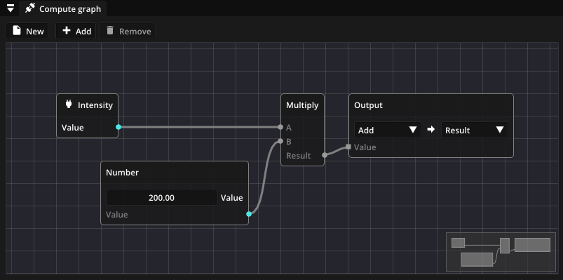
One example of a node is the Multiply node. The pins on the left side represent the inputs of the node, while the pin on the right represents its output. These input and output pins need to be connected to the rest of the compute graph. For example, the Multiply node could be used to scale the Intensity input by a fixed number to compute a final particle count. To implement this behavior, one input pin of the Multiply is connected to the Intensity input node and the other input pin to a Number constant node, where the scaling factor can be set. The output pin of the Multiply node is then connected to the output node.
The output node of a compute graph is a special node that decides how the particle property is set based on the incoming data. In the simplest case the value of the compute graph directly sets the particle property. But can also choose to Add or to Multiply the compute graph value with the existing value of the particle property set in the Properties window. If the property is an animated property, you additionally have the option to set a specific keyframe of the animation.
Creating compute graphs
You can add new nodes by dragging a node from the toolbox on the right and dropping it on the graph or by clicking Add in the toolbar. The list of available nodes can be filtered by typing in the search box at the top.
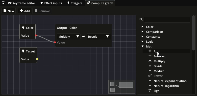
Another way to create nodes is to drag out a node pin and then letting go. This will show a popup of available nodes. After selecting a node type, a new node is created. Using this method, there are several keyboard shortcuts for creating common node types directly.
Shortcut |
Node |
|---|---|
1 |
Number |
2 |
Vector 2 |
3 |
Vector 3 |
4 |
Vector 4 |
B |
Boolean |
I |
Integer |
C |
Color |
After adding a new node, connect its input and output pins to the rest of the graph by dragging out links from each pin. The pin color and shape denote the data type that is expected for the attribute. To remove a node, select the node(s) and press Del or click Remove in the tool bar.
Available nodes
Constants
Node |
Inputs |
Description |
|---|---|---|
Boolean |
Boolean constant, which can be true or false. |
|
Integer |
Integer constant, which can be any positive or negative integer. |
|
Number |
Number constant, which can be any rational number. |
|
Vector 2 |
Vector constant with two components. |
|
Vector 3 |
Vector constant with three components. |
|
Vector 4 |
Vector constant with four components. |
|
Color |
Color constant with four components (RGBA). |
Colors
Node |
Inputs |
Description |
|---|---|---|
Blend |
A, B |
Blends colors A and B together using the specified blending mode. |
Color ramp |
Value |
Picks a color from the specified gradient using Value as an index between 0.0 and 1.0. |
Adjust brightness |
Color, Brightness |
Increases the brightness of Color for Brightness > 0 and decreases it for Brightness < 0. |
Adjust exposure |
Color, Exposure |
Increases the exposure of Color for Exposure > 0 and decreases it for Exposure < 0. |
Adjust contrast |
Color, Contrast |
Increases the contrast of Color for Contrast > 0 and decreases it for Contrast < 0. |
Adjust saturation |
Color, Saturation |
Increases the saturation of Color for Saturation > 0 and decreases it for Saturation < 0. |
Posterize |
Color, Number |
Reduces the number of available colors per channel to Number. |
Math
Node |
Inputs |
Description |
|---|---|---|
Add |
A, B |
Adds A and B (A + B). |
Subtract |
A, B |
Subtracts B from A (A - B). |
Multiply |
A, B |
Multiplies A with B (A * B). |
Divide |
A, B |
Divides A by B (A / B). |
Modulo |
A, B |
Computes the modulus of A and B (A mod B). |
Power |
A, B |
Raises A to the power of B (A^B). |
Natural exponentiation |
Value |
Computes the natural exponentiation of Value (exp(Value)). |
Natural logarithm |
Value |
Computes the natural logarithm of Value (ln(Value)). |
Sign |
Value |
Returns the sign of Value, i.e. +1 if Value is positive, -1 if Value is negative and 0 if Value is 0. |
Absolute value |
Value |
Returns the absolute value of Value (|Value|). |
Min |
A, B |
Returns the minimum of A and B (min(A, B)). |
Max |
A, B |
Returns the maximum of A and B (max(A, B)). |
Clamp |
Value, Min, Max |
Limits Value to the range [Min, Max]. |
Linear interpolation |
A, B, Factor |
Interpolations linearly between A and B using Factor (in the range [0, 1]). |
Floor |
Value |
Rounds Value down to the next integer. |
Ceil |
Value |
Rounds Value up to the next integer. |
Round |
Value |
Rounds Value to the nearest integer. |
Square root |
Value |
Computes the square root of Value. |
Sin |
Value |
Computes the sine of Value. |
Cos |
Value |
Computes the cosine of Value. |
Arcsin |
Value |
Computes the arcus sine of Value. |
Arccos |
Value |
Computes the arcus cosine of Value. |
Dot product |
A, B |
Computes the dot product of vectors A and B. |
Cross product |
A, B |
Computes the cross product of vectors A and B. |
Normalize |
Vector |
Normalizes Vector to a vector of length 1. |
Vector length |
Vector |
Returns the length or magnitude of Vector. |
Step |
Value, Edge |
Generates a step function by comparing Value to Edge. If Value < Edge, the output is 0 and otherwise 1. |
Smooth step |
Value, Edge 1, Edge 2 |
Performs a smooth interpolation between 0 and 1 when Edge 1 < Value < Edge 2. |
Logic
Node |
Inputs |
Description |
|---|---|---|
Negation (NOT) |
Value |
Negates the boolean Value. |
Conjunction (AND) |
A, B |
Outputs true if and only if both A and B are true. |
Disjunction (OR) |
A, B |
Outputs true if and only if A or B is true. |
Exclusive disjunction (XOR) |
A, B |
Outputs true if and only if either A or B is true. |
Branch |
Predicate, True, False |
Outputs the value for True if Predicate evaluates to true and the value for False otherwise. |
Comparison
Node |
Inputs |
Description |
|---|---|---|
Equal |
A, B |
Outputs true if A = B and false otherwise. |
Not equal |
A, B |
Outputs true if A ≠ B and false otherwise. |
Approximately equal |
A, B |
Outputs true if A ≈ B (depending on given Epsilon) and false otherwise. |
Less |
A, B |
Outputs true if A < B and false otherwise. |
Less or equal |
A, B |
Outputs true if A ≤ B and false otherwise. |
Greater |
A, B |
Outputs true if A > B and false otherwise. |
Greater or equal |
A, B |
Outputs true if A ≥ B and false otherwise. |
Utility
Node |
Inputs |
Description |
|---|---|---|
Value curve |
Value |
Defines a graph using keyframes and samples this graph at position Value. |
Split vector (2) |
Vector |
Splits the two-dimensional vector Vector into its components. |
Split vector (3) |
Vector |
Splits the three-dimensional vector Vector into its components. |
Split vector (4) |
Vector |
Splits the four-dimensional vector Vector into its components. |
Merge vector (2) |
X, Y |
Combines X, Y into a two-dimensional vector. |
Merge vector (3) |
X, Y, Z |
Combines X, Y, Z into a three-dimensional vector. |
Merge vector (4) |
X, Y, Z, W |
Combines X, Y, Z, W into a four-dimensional vector. |